Spatial BayesSpace Branch
Spatial clustering, subspot enhancement, and marker imputation with BayesSpace
What it does
This workflow applies BayesSpace to spatial transcriptomics data for spatial clustering and subspot-level resolution enhancement. The committed materials cover SingleCellExperiment preparation, cluster-number tuning, spatial clustering, enhanced-resolution modeling, marker-gene imputation, and inspection of saved MCMC chains.
When to use it
Use this workflow when the main question is spatial domain structure at or below spot resolution and you want a Bayesian spatial model rather than a purely Seurat-style clustering workflow. It is most useful for ST or Visium-like datasets where cluster smoothing, subspot enhancement, and marker-expression imputation are the goals.
Prerequisites
- Source folder:
ST_BayesSpace_branch - Main files:
README.mdST_BayesSpace.rmd- rendered reference:
ST_BayesSpace.html
- Committed figures in
ST_BayesSpace_branch/figures - Required packages include
BayesSpace,SingleCellExperiment, andggplot2
Steps
Load a spatial experiment into a SingleCellExperiment
The notebook starts by describing the three accepted entry paths for BayesSpace: readVisium() for Space Ranger outputs, getRDS() for packaged examples, or manual SingleCellExperiment construction from counts plus row/column metadata.
melanoma <- getRDS(dataset = "2018_thrane_melanoma", sample = "ST_mel1_rep2")That example dataset is then used for the rest of the committed tutorial.
Preprocess the experiment and choose the number of clusters
BayesSpace’s helper preprocessing step log-normalizes if needed, keeps highly variable genes, and stores principal components for downstream modeling. The tutorial then uses qTune() and qPlot() to choose q, the number of spatial clusters.
set.seed(102)
melanoma <- spatialPreprocess(
  melanoma,
  platform = "ST",
  n.PCs = 7,
  n.HVGs = 2000,
  log.normalize = FALSE
)

melanoma <- qTune(melanoma, qs = seq(2, 10), platform = "ST", d = 7)
qPlot(melanoma)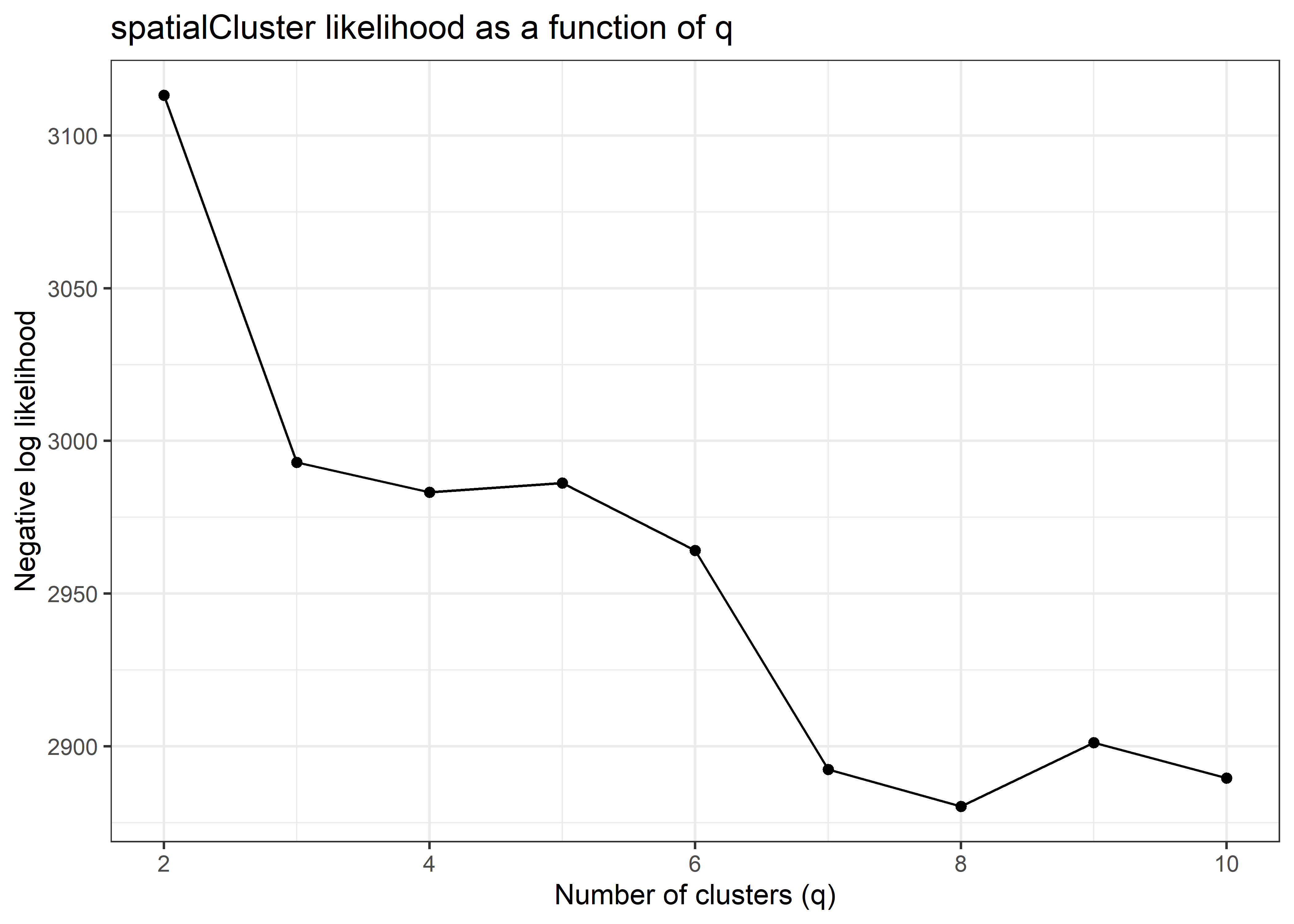
Run spatial clustering and inspect the resulting domains
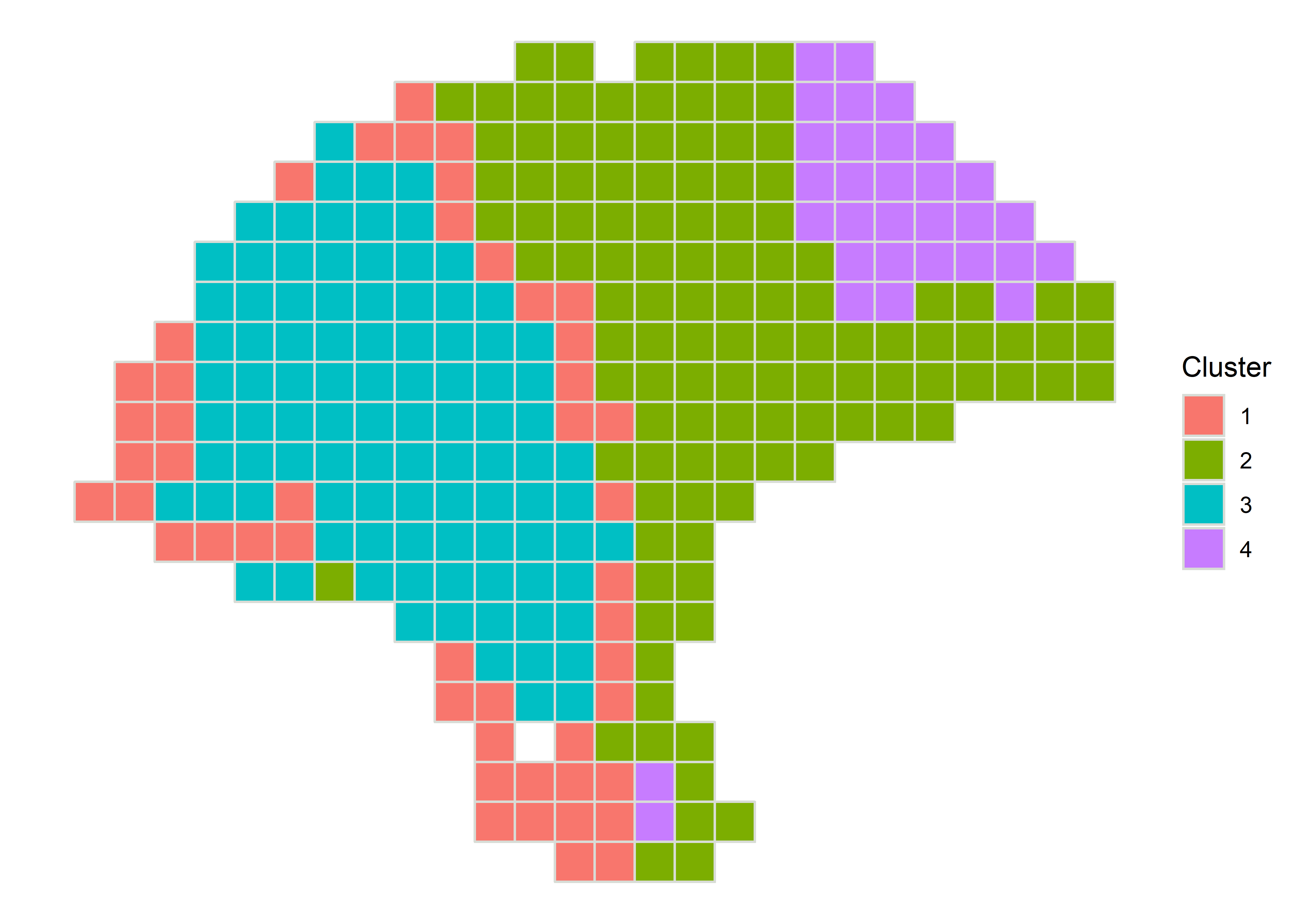
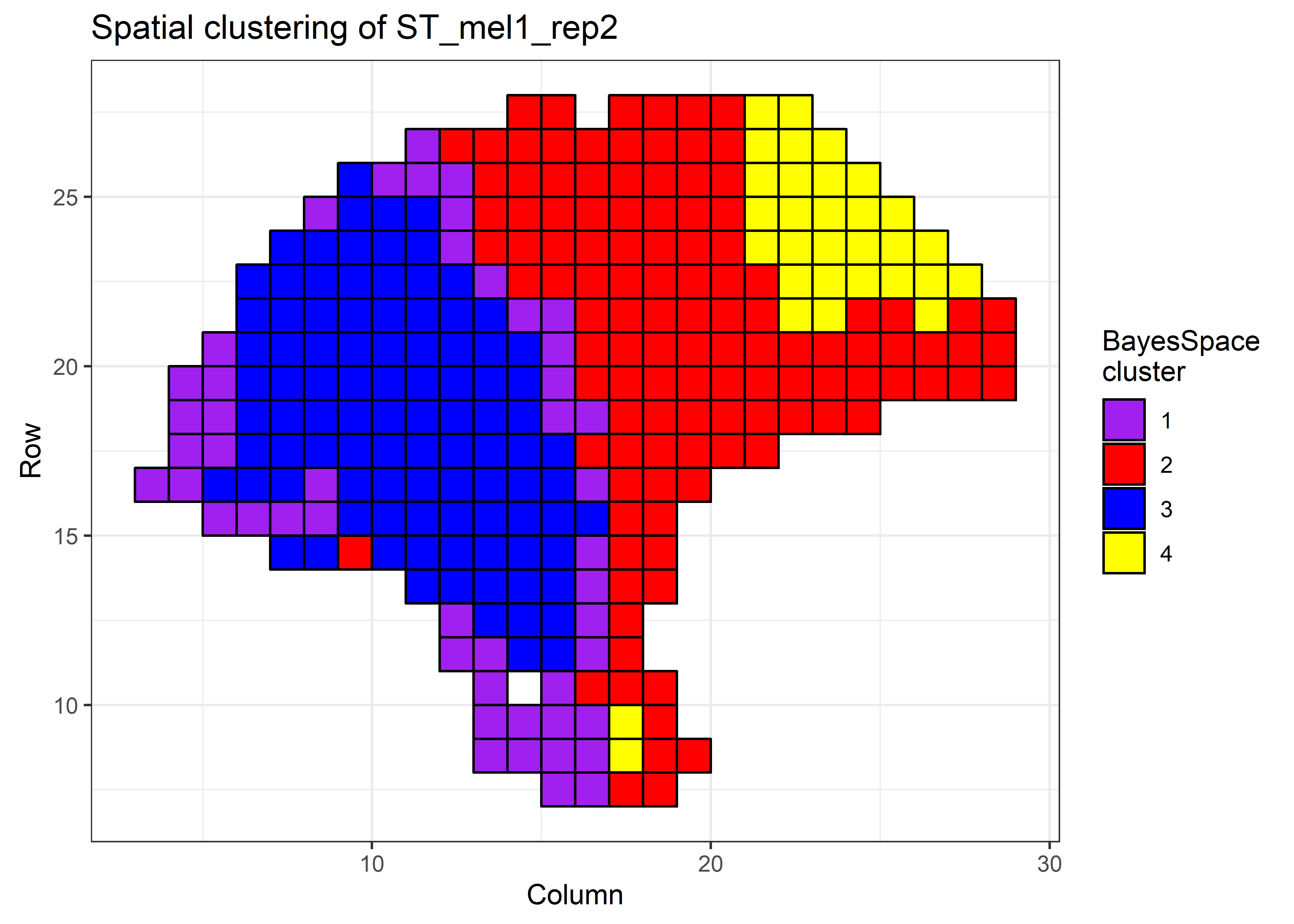
Once q is selected, the workflow runs spatialCluster() with a spatial prior and stores both the initialization and the final BayesSpace cluster assignments in colData.
set.seed(149)
melanoma <- spatialCluster(
  melanoma,
  q = 4,
  platform = "ST",
  d = 7,
  init.method = "mclust",
  model = "t",
  gamma = 2,
  nrep = 1000,
  burn.in = 100,
  save.chain = TRUE
)
The committed figures show both the default spatial cluster plot and a customized version with explicit colors and borders.
Enhance resolution to the subspot level
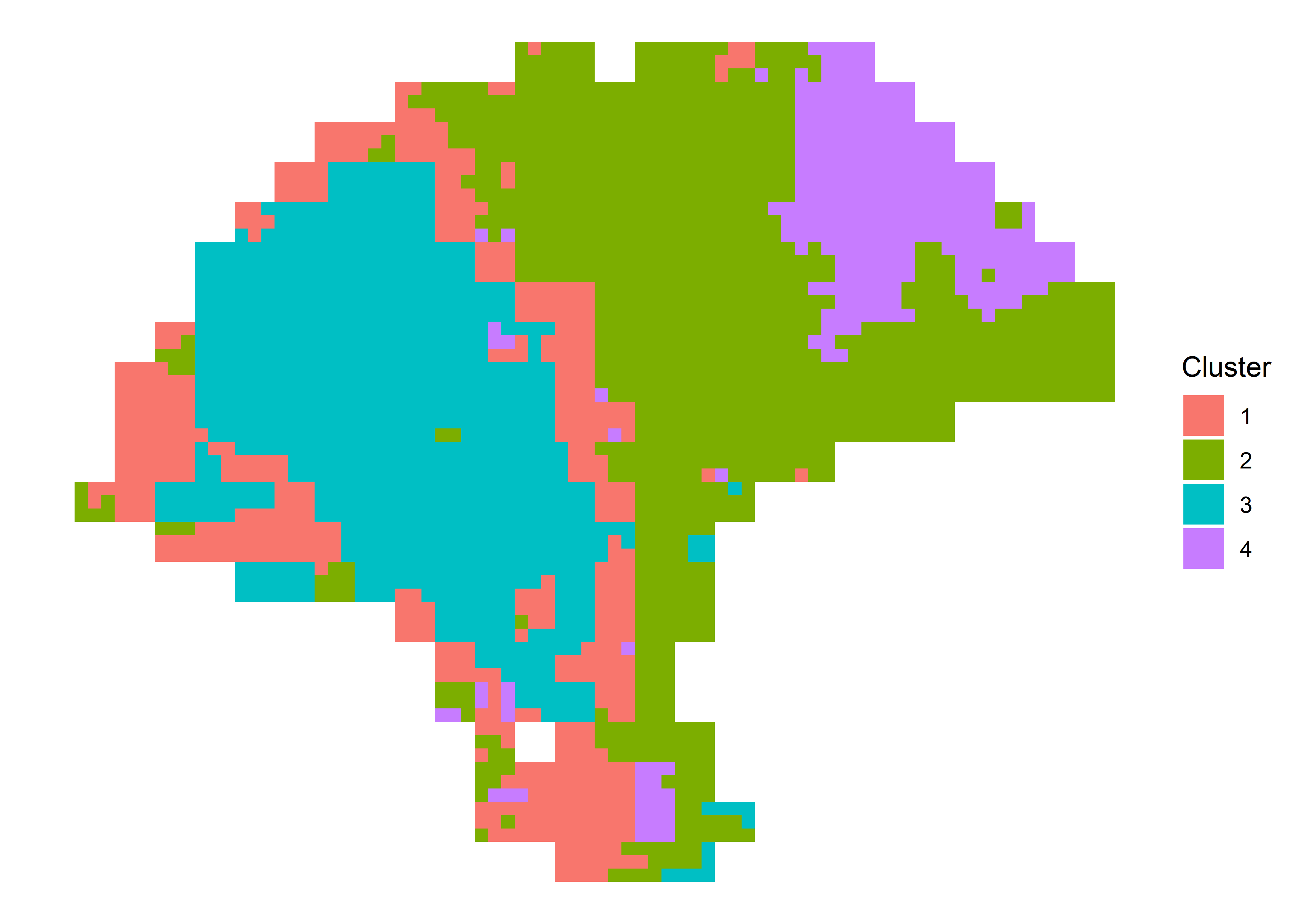
The next branch runs spatialEnhance() to infer subspot-level principal components and cluster assignments. This is one of the main reasons to use BayesSpace over a simpler spatial clustering workflow.
melanoma.enhanced <- spatialEnhance(
  melanoma,
  q = 4,
  platform = "ST",
  d = 7,
  model = "t",
  gamma = 2,
  jitter_prior = 0.3,
  jitter_scale = 3.5,
  nrep = 1000,
  burn.in = 100,
  save.chain = TRUE
)
Impute marker-gene expression and compare spot versus subspot views
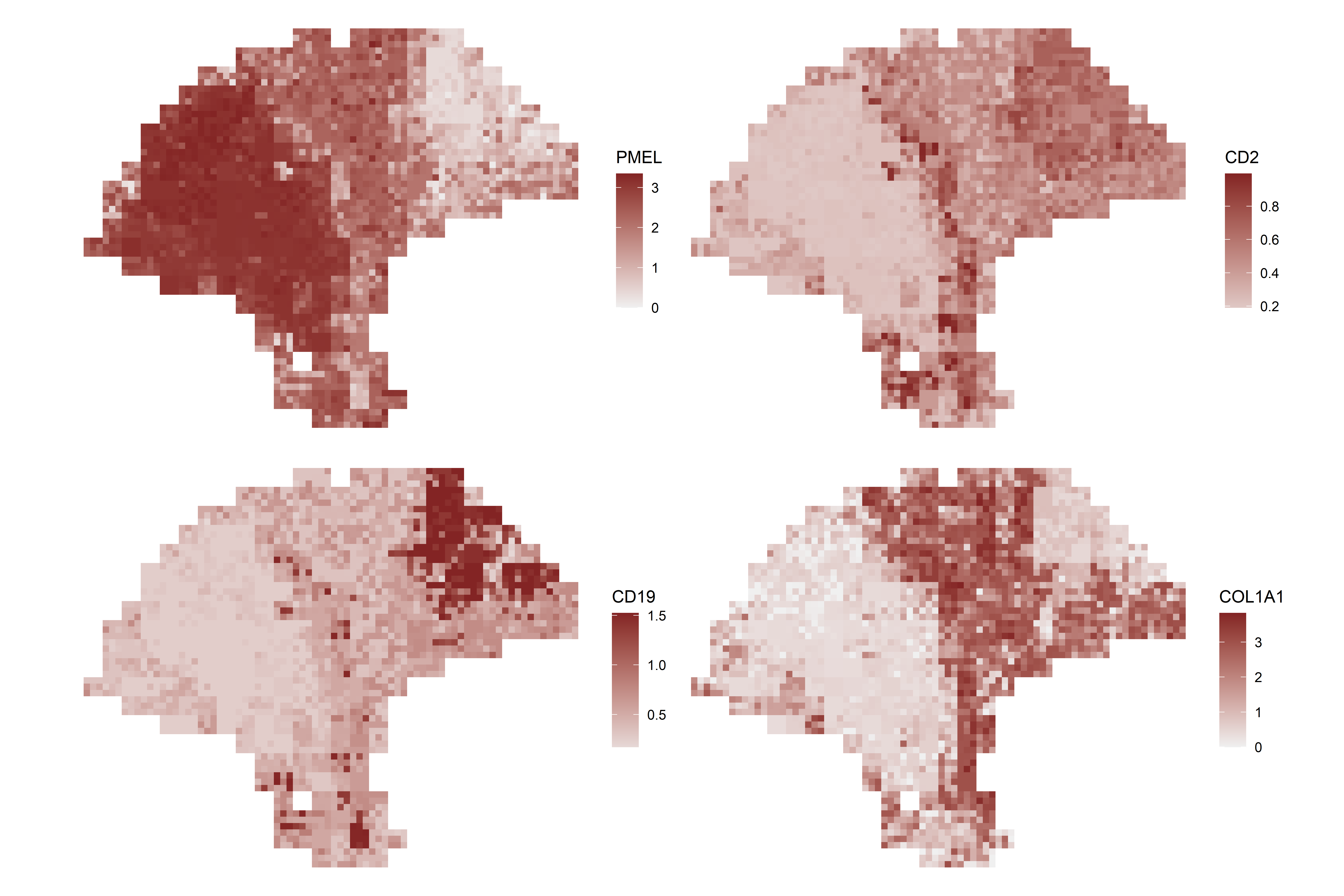
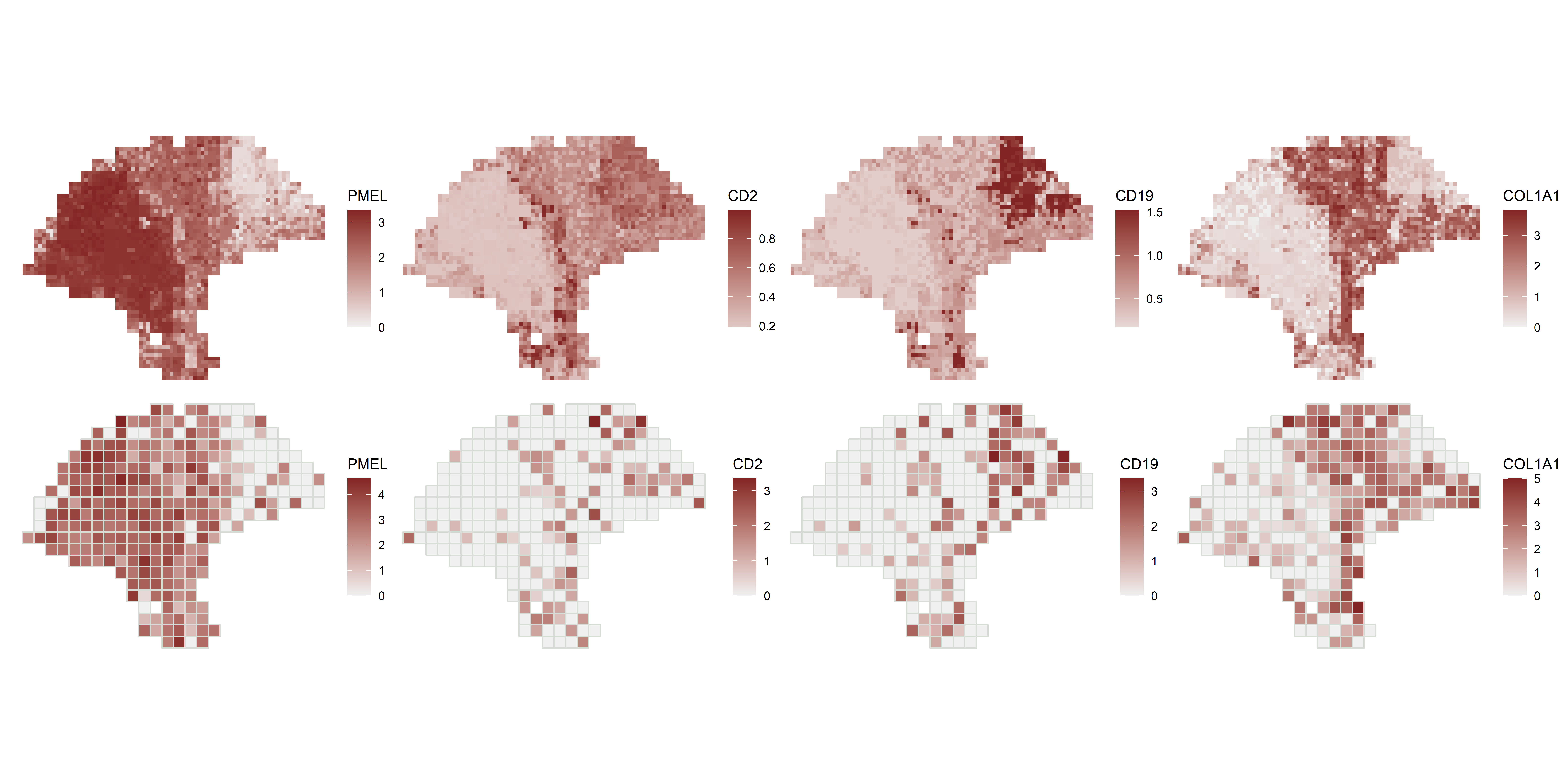
Because BayesSpace enhances PCs rather than gene counts directly, the tutorial next uses enhanceFeatures() to impute selected marker genes at subspot resolution.
markers <- c("PMEL", "CD2", "CD19", "COL1A1")
melanoma.enhanced <- enhanceFeatures(
  melanoma.enhanced,
  melanoma,
  feature_names = markers,
  nrounds = 0
)
The committed figures then compare enhanced marker expression panels with the original spot-level views.
Inspect saved Markov chains when needed
The notebook closes by documenting how to read the saved MCMC chain with mcmcChain() when save.chain = TRUE, or remove it with removeChain().
chain <- mcmcChain(melanoma)
chain[1:5, 1:5]
This is a useful workflow-specific detail because BayesSpace exposes its iterative Bayesian fit in a way that the other spatial branches do not.
Gotchas / notes
- The demo reduces iteration counts for runtime, but the committed notebook explicitly recommends much larger
nrepvalues for real analyses. - Enhancement relies on principal components and then imputes expression afterward; it does not directly model subspot gene counts from the start.
- The README refers to a differently named Rmd in one place, but the committed executable tutorial file in this repo is
ST_BayesSpace.rmd. - The bundled example data are specific to the BayesSpace tutorial; readers using Visium outputs should switch to
readVisium().